Summarize
Summarizing EMS data
Notebook of summary statistics using simulated EMS data.
This Jupyter Notebook is designed to demonstrate how you can characterize the "shape" of the data, e.g. basic counts and summaries.
Import libraries
Libaries add functionality to Python. Polars and Pandas are currently the main libraries for data science in Python. With these libraries, you import your data into "dataframes" (df) that are like mini spreadsheets.
I recently switched to Polars after a decade using Pandas (June 2023).
Libaries
- Polars: An ultra-fast, df-based statistics library, written in Rust
- Pandas: Pandas brought dataframe constructs to Python. This allowed me to replace R as my main scripting language
- Numpy: (Numerical Python) does the underlying math.
- Matplotlib does the graphing (Thanks for everything John H. - RIP)
- Plotly is a visualization library (used for both graphs and pretty tables)
- Datetime is a module for handling dates and times, it provides useful things like adding and subtracting dates to calculate duration.
import polars as pl
import pandas as pd
import numpy as np
import matplotlib
import matplotlib.pyplot as plt
import plotly.express as px
from datetime import datetime
This is a handy script for making wider, more legible, table columns in the Notebook.
pl.Config.set_fmt_str_lengths(50)
Naming conventions
These are useful fot making your code interoperable. You can assign variables, modules, and libraries to whatever name you want--however, standard names are best practice.
- df = dataframe
- pl = polars
- pd = pandas
- px = plotly express
- np = numpy
- plt = pyplot (matplotlib)
Simulate the data
The simulation chapter explains the function of this script. I often simulate data in health care. It saves you the grief of privacy. You write most of the code while you wait for data access. In research it is good practice to understand your statisics before you conduct your study. By simulating you can determine the sample size and types of questions you should ask. Simulation can provide unique insights and baselines for future analysis. It can also allow you to model your system in alternate future states.
Here we call the simulate script in another Jupyter notebook using the magic function "%run":
%run ./simulate.ipynb
Load the data
Comma-seperated values (csv) are among the most useful file formats for data science. They're simply column values seperated by commas, e.g. value1, value2, value 3. They can be opened with any spreadsheet software, e.g. Excel or Google Sheets. Here we use the read_csv command and useful function "try_parse_dates" to convert any date columns to "datetime".
df = pl.read_csv('data/events.csv', try_parse_dates=True)
Summarize the "shape" of the data
df.shape
The command ".head( )" allows you to display a subset N of rows of the data you loaded.
The command ".to_pandas()" is used to convert a Polars df to a Pandas df. It providers a more attractive/legible output.
df.head(3).to_pandas()
| event_id | dtime_event | dtime_page | dtime_arrived | dtime_transport | dtime_dest | pt_id | mpds_code | mpds_name | impression_code | ... | bp_dia_first | bp_dia_last | temp_first | temp_last | pain_first | pain_last | bgl_first | bgl_last | gcs_first | gcs_last | |
|---|---|---|---|---|---|---|---|---|---|---|---|---|---|---|---|---|---|---|---|---|---|
| 0 | 100559 | 2023-01-01 01:26:34.515957 | 2023-01-01 01:31:34.515957 | 2023-01-01 01:36:34.515957 | 2023-01-01 01:39:34.515957 | 2023-01-01 01:44:34.515957 | id-3468436uno | 10 | Chest Pain | 4 | ... | 137 | 129 | 36.8 | 36.6 | 1 | 3 | 5.3 | 5.7 | 14 | 12 |
| 1 | 101371 | 2023-01-01 03:32:41.574836 | 2023-01-01 03:40:41.574836 | 2023-01-01 03:42:41.574836 | 2023-01-01 03:51:41.574836 | 2023-01-01 03:55:41.574836 | id-0133733oag | 31 | Subject Unconscious | 7 | ... | 52 | 58 | 36.0 | 36.2 | 0 | 0 | 3.5 | 3.3 | 6 | 5 |
| 2 | 102061 | 2023-01-01 07:05:06.322297 | 2023-01-01 07:11:06.322297 | 2023-01-01 07:15:06.322297 | 2023-01-01 07:25:06.322297 | 2023-01-01 07:32:06.322297 | id-3757177vdh | 10 | Chest Pain | 4 | ... | 109 | 118 | 36.8 | 36.5 | 8 | 10 | 5.1 | 4.6 | 15 | 14 |
3 rows × 27 columns
Data Types
Inspect the "types" of data in each column with "df.dtypes".
Notice the datetimes were created on import. Many of the early challenges you will encounter relate to the type of data, e.g. trying to subtract strings without converting them to integers.
The main data types are:
- Datetime (date and/or time, e.g. 2023-01-01 05:07:45.135653)
- Int64 (Integer e.g. 911)
- Utf8 (string e.g. "John Smith")
- Float64 (float e.g. 36.5)
- Boolean (True/False)
df.dtypes
Slice the data
Use square brackets and comma-: syntax to slice the data.
df[1,:].to_pandas()
| event_id | dtime_event | dtime_page | dtime_arrived | dtime_transport | dtime_dest | pt_id | mpds_code | mpds_name | impression_code | ... | bp_dia_first | bp_dia_last | temp_first | temp_last | pain_first | pain_last | bgl_first | bgl_last | gcs_first | gcs_last | |
|---|---|---|---|---|---|---|---|---|---|---|---|---|---|---|---|---|---|---|---|---|---|
| 0 | 101371 | 2023-01-01 03:32:41.574836 | 2023-01-01 03:40:41.574836 | 2023-01-01 03:42:41.574836 | 2023-01-01 03:51:41.574836 | 2023-01-01 03:55:41.574836 | id-0133733oag | 31 | Subject Unconscious | 7 | ... | 52 | 58 | 36.0 | 36.2 | 0 | 0 | 3.5 | 3.3 | 6 | 5 |
1 rows × 27 columns
Slice the columns by name. This is useful for creating a sub dataframe. Here we slice all times columns for the 911 events.
df[:,['event_id','dtime_event','dtime_page','dtime_arrived','dtime_transport','mpds_name']].head(3).to_pandas()
| event_id | dtime_event | dtime_page | dtime_arrived | dtime_transport | mpds_name | |
|---|---|---|---|---|---|---|
| 0 | 100559 | 2023-01-01 01:26:34.515957 | 2023-01-01 01:31:34.515957 | 2023-01-01 01:36:34.515957 | 2023-01-01 01:39:34.515957 | Chest Pain |
| 1 | 101371 | 2023-01-01 03:32:41.574836 | 2023-01-01 03:40:41.574836 | 2023-01-01 03:42:41.574836 | 2023-01-01 03:51:41.574836 | Subject Unconscious |
| 2 | 102061 | 2023-01-01 07:05:06.322297 | 2023-01-01 07:11:06.322297 | 2023-01-01 07:15:06.322297 | 2023-01-01 07:25:06.322297 | Chest Pain |
Filter the data
Filtering is useful for subsetting rows. For example here we filter a dataframe for only the events (rows) that were coded as "strokes" by the dispatcher.
df.filter(df['mpds_name']=="Stroke").head(3).to_pandas()
| event_id | dtime_event | dtime_page | dtime_arrived | dtime_transport | dtime_dest | pt_id | mpds_code | mpds_name | impression_code | ... | bp_dia_first | bp_dia_last | temp_first | temp_last | pain_first | pain_last | bgl_first | bgl_last | gcs_first | gcs_last | |
|---|---|---|---|---|---|---|---|---|---|---|---|---|---|---|---|---|---|---|---|---|---|
| 0 | 108123 | 2023-01-02 14:59:08.432350 | 2023-01-02 15:01:08.432350 | 2023-01-02 15:05:08.432350 | 2023-01-02 15:14:08.432350 | 2023-01-02 15:23:08.432350 | id-9927980zad | 28 | Stroke | 11 | ... | 105 | 105 | 36.0 | 36.0 | 2 | 2 | 4.9 | 5.1 | 13 | 10 |
| 1 | 108485 | 2023-01-02 20:27:54.993135 | 2023-01-02 20:32:54.993135 | 2023-01-02 20:34:54.993135 | 2023-01-02 20:45:54.993135 | 2023-01-02 20:51:54.993135 | id-4150367wce | 28 | Stroke | 11 | ... | 118 | 103 | 36.6 | 36.4 | 0 | 0 | 4.9 | 4.4 | 5 | 3 |
| 2 | 115318 | 2023-01-04 20:21:51.956753 | 2023-01-04 20:30:51.956753 | 2023-01-04 20:38:51.956753 | 2023-01-04 20:47:51.956753 | 2023-01-04 20:51:51.956753 | id-8886685sji | 28 | Stroke | 11 | ... | 40 | 41 | 37.5 | 37.6 | 1 | 1 | 5.3 | 5.4 | 13 | 12 |
3 rows × 27 columns
Here is a different syntax pl.col for doing the same thing. This is considered better practice. pl.col stands for polars column. Note the double equal signs for an equality operator.
df.filter(pl.col("mpds_name")=="Stroke").head(3).to_pandas()
| event_id | dtime_event | dtime_page | dtime_arrived | dtime_transport | dtime_dest | pt_id | mpds_code | mpds_name | impression_code | ... | bp_dia_first | bp_dia_last | temp_first | temp_last | pain_first | pain_last | bgl_first | bgl_last | gcs_first | gcs_last | |
|---|---|---|---|---|---|---|---|---|---|---|---|---|---|---|---|---|---|---|---|---|---|
| 0 | 108123 | 2023-01-02 14:59:08.432350 | 2023-01-02 15:01:08.432350 | 2023-01-02 15:05:08.432350 | 2023-01-02 15:14:08.432350 | 2023-01-02 15:23:08.432350 | id-9927980zad | 28 | Stroke | 11 | ... | 105 | 105 | 36.0 | 36.0 | 2 | 2 | 4.9 | 5.1 | 13 | 10 |
| 1 | 108485 | 2023-01-02 20:27:54.993135 | 2023-01-02 20:32:54.993135 | 2023-01-02 20:34:54.993135 | 2023-01-02 20:45:54.993135 | 2023-01-02 20:51:54.993135 | id-4150367wce | 28 | Stroke | 11 | ... | 118 | 103 | 36.6 | 36.4 | 0 | 0 | 4.9 | 4.4 | 5 | 3 |
| 2 | 115318 | 2023-01-04 20:21:51.956753 | 2023-01-04 20:30:51.956753 | 2023-01-04 20:38:51.956753 | 2023-01-04 20:47:51.956753 | 2023-01-04 20:51:51.956753 | id-8886685sji | 28 | Stroke | 11 | ... | 40 | 41 | 37.5 | 37.6 | 1 | 1 | 5.3 | 5.4 | 13 | 12 |
3 rows × 27 columns
Here we assign the results to a new df called df_strokes so we can reuse the stroke values for future calculations. Note: it is convention to put the object type before the name, e.g. df_name for a dataframe.
df_strokes = df.filter(pl.col("mpds_name")=="Stroke")
Here we use datetime and the "with_columns" operators to quickly calculate the event duration.
df_strokes = df_strokes.with_columns([
    (pl.col("dtime_dest")-pl.col("dtime_event")).alias("event_duration")
])
df_strokes['event_duration'].head(3)
| event_duration |
|---|
| duration[μs] |
| 24m |
| 24m |
| 30m |
Sample data
The "sample" command is useful for pulling a random set from the dataframe. This can be useful when QA'ing the data, taking a quick look, or even choosing a training set for a model.
df.sample(3).to_pandas()
| event_id | dtime_event | dtime_page | dtime_arrived | dtime_transport | dtime_dest | pt_id | mpds_code | mpds_name | impression_code | ... | bp_dia_first | bp_dia_last | temp_first | temp_last | pain_first | pain_last | bgl_first | bgl_last | gcs_first | gcs_last | |
|---|---|---|---|---|---|---|---|---|---|---|---|---|---|---|---|---|---|---|---|---|---|
| 0 | 422035 | 2023-04-08 12:26:55.252636 | 2023-04-08 12:31:55.252636 | 2023-04-08 12:35:55.252636 | 2023-04-08 12:41:55.252636 | 2023-04-08 12:45:55.252636 | id-3052353suv | 12 | Seizures | 8 | ... | 71 | 69 | 37.2 | 37.0 | 5 | 7 | 3.3 | 3.3 | 14 | 14 |
| 1 | 465293 | 2023-04-23 09:28:52.166148 | 2023-04-23 09:35:52.166148 | 2023-04-23 09:42:52.166148 | 2023-04-23 09:49:52.166148 | 2023-04-23 09:54:52.166148 | id-3016394fbw | 31 | Subject Unconscious | 7 | ... | 117 | 128 | 37.7 | 37.4 | 2 | 0 | 3.8 | 3.9 | 9 | 10 |
| 2 | 294131 | 2023-02-25 15:58:18.257116 | 2023-02-25 16:08:18.257116 | 2023-02-25 16:15:18.257116 | 2023-02-25 16:19:18.257116 | 2023-02-25 16:28:18.257116 | id-7906369mbj | 13 | Diabetic Problems | 10 | ... | 64 | 55 | 37.3 | 37.3 | 0 | 0 | 2.2 | 2.1 | 14 | 14 |
3 rows × 27 columns
SQL style select
You can use a Structured Query Language (SQL) style to query your data via the "select command".
df.select(['mpds_code','mpds_name']).head(3)
| mpds_code | mpds_name |
|---|---|
| i64 | str |
| 10 | "Chest Pain" |
| 31 | "Subject Unconscious" |
| 10 | "Chest Pain" |
Similarly you could retreive all the cardiac related events. Here we use "is_in" to retrieve rows that are either "Cardiac Arrest" or "Heart Problem".
# Cardiac events
df.filter(
    pl.col("mpds_name").is_in(["Cardiac Arrest","Heart Problem"])
).head(3).to_pandas()
| event_id | dtime_event | dtime_page | dtime_arrived | dtime_transport | dtime_dest | pt_id | mpds_code | mpds_name | impression_code | ... | bp_dia_first | bp_dia_last | temp_first | temp_last | pain_first | pain_last | bgl_first | bgl_last | gcs_first | gcs_last | |
|---|---|---|---|---|---|---|---|---|---|---|---|---|---|---|---|---|---|---|---|---|---|
| 0 | 108638 | 2023-01-02 22:20:37.847541 | 2023-01-02 22:29:37.847541 | 2023-01-02 22:33:37.847541 | 2023-01-02 22:36:37.847541 | 2023-01-02 22:46:37.847541 | id-4095716qsv | 9 | Cardiac Arrest | 13 | ... | 116 | 98 | 36.2 | 36.1 | 0 | 0 | 6.9 | 6.4 | 12 | 15 |
| 1 | 109215 | 2023-01-03 06:50:53.671638 | 2023-01-03 06:56:53.671638 | 2023-01-03 07:00:53.671638 | 2023-01-03 07:11:53.671638 | 2023-01-03 07:18:53.671638 | id-7502291xuj | 9 | Cardiac Arrest | 13 | ... | 115 | 100 | 36.9 | 37.1 | 0 | 1 | 6.0 | 6.4 | 6 | 9 |
| 2 | 110282 | 2023-01-03 11:47:45.327361 | 2023-01-03 11:51:45.327361 | 2023-01-03 11:53:45.327361 | 2023-01-03 11:58:45.327361 | 2023-01-03 12:04:45.327361 | id-4735630woq | 19 | Heart Problem | 12 | ... | 125 | 133 | 36.8 | 37.1 | 10 | 10 | 6.0 | 5.7 | 14 | 15 |
3 rows × 27 columns
Unique values
Often you may want to count the unique values e.g. numer of unique patients, where you may have seen the same patient multiple times. You can also use unique to generate custom lists based on values you've seen, e.g. impression codes.
df.select([
    pl.col("impression_name").n_unique()

])
| impression_name |
|---|
| u32 |
| 18 |
Groupby
This is one of the most useful tools. They are similar to pivot tables. Here we count the number of calls for each impression type.
df.groupby("impression_name").count()
| impression_name | count |
|---|---|
| str | u32 |
| "Hyperthermia" | 51 |
| "Poisoning or drug ingestion" | 61 |
| "Cardiac rhythm disturbance" | 54 |
| "Diabetic symptoms hyperglycemia" | 69 |
| "Altered level of consciousness" | 55 |
| "Abdominal pain or problems" | 64 |
| "Chest pain or discomfort" | 51 |
| "Hypothermia" | 52 |
| "Loss of consciousness or fainting" | 53 |
| "Stroke or cerebrovascular accident CVA" | 62 |
| "Behavioral or psychiatric disorder" | 59 |
| "Respiratory distress" | 47 |
| "Seizure" | 56 |
| "Other" | 53 |
| "Diabetic symptoms hypoglycemia" | 51 |
| "Traumatic injury" | 56 |
| "Cardiac arrest" | 55 |
| "Allergic reaction" | 51 |
Summary statistics
Now we actually starting to calculate some stats. Here we use moments such as max and min to evaluate the spread of our data.
df.select([
    pl.col("age").min().alias("min"),
    pl.col("age").max().alias("max"),
    pl.col("age").mean().alias("mean"),
    pl.col("age").median().alias("median"),
    pl.col("age").std().alias("std dev")
])
| min | max | mean | median | std dev |
|---|---|---|---|---|
| i64 | i64 | f64 | f64 | f64 |
| 0 | 106 | 61.054 | 66.0 | 25.707936 |
This is so useful that there is a built-in function called "describe." This is one of the first things I do when looking at data. It's a great way to find outliers, or ensure you've got the right numbers and they make intuitive sense.
df.select([
    pl.col("age")
]).describe()
| describe | age |
|---|---|
| str | f64 |
| "count" | 1000.0 |
| "null_count" | 0.0 |
| "mean" | 61.054 |
| "std" | 25.707936 |
| "min" | 0.0 |
| "max" | 106.0 |
| "median" | 66.0 |
| "25%" | 42.0 |
| "75%" | 82.0 |
Select a column
Here we use select to isolate one column of data. We want to look the age distruction of our patient community.
age = df.select([
    pl.col("age")
])
Random sample of data
age.sample(10)
| age |
|---|
| i64 |
| 86 |
| 64 |
| 42 |
| 55 |
| 4 |
| 23 |
| 81 |
| 81 |
| 83 |
| 74 |
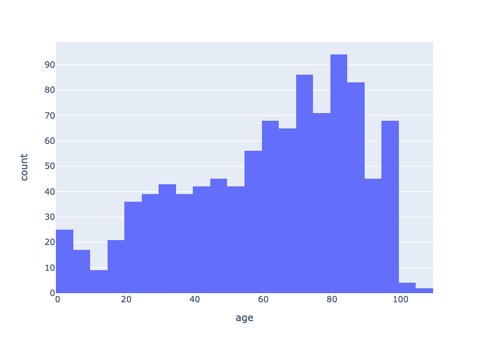
Vizualise the data
With one command we can generate an age histogram. This shape is farily representative of our EMS patient community.
plt.hist(age)
plt.show()

Graph with plotly
Plotly provides more attractive outputs. With enough tweaking you can generate camera-ready graphics or interactive dashboards. We'll get into visualizations in more detail in the visualizing chapter.
fig = px.histogram(age, x="age", nbins=30)
fig.show(renderer="svg")

fig.show(renderer="png")
Casting and modifying values
Here we cast an integer to string and add text. This can be useful for labeling figures or creating identifier keys.
# Modify an integer column by casting to string and adding text
df = df.with_columns([
    (pl.col("age").cast(pl.Utf8)+ " years old").alias("age_text"),
    (pl.col("dtime_dest")-pl.col("dtime_event")).alias("duration")
])
And now we add columns with mean values. This can be used to observe deviation from the mean and look for patterns. This is starting to look useful.
df=df.with_columns([
    pl.all(),
    pl.col("age").mean().alias("age_mean"),
    pl.col("duration").mean().alias("duration_mean")
])
df[:,['event_id','mpds_name', 'age','age_mean', 'duration', 'duration_mean']].head(3).to_pandas()
| event_id | mpds_name | age | age_mean | duration | duration_mean | |
|---|---|---|---|---|---|---|
| 0 | 100559 | Chest Pain | 46 | 61.054 | 0 days 00:18:00 | 0 days 00:25:30 |
| 1 | 101371 | Subject Unconscious | 27 | 61.054 | 0 days 00:23:00 | 0 days 00:25:30 |
| 2 | 102061 | Chest Pain | 85 | 61.054 | 0 days 00:27:00 | 0 days 00:25:30 |
Pivot the data
Grouping approaches such as ".over()" can be used to group and summarize. For example, here we calculate the mean age by MPDS call. If the data was real, we'd probably expect to see a differnce in age by call, e.g. geriatric versus pediatric conditions.
df = df.with_columns([
    pl.col("age").mean().over("mpds_name").alias("age_by_mpds"),
    pl.col("duration").mean().over("mpds_name").alias("duration_by_mpds")
])
df.select(pl.col("age_by_mpds", "mpds_name")).unique()
| age_by_mpds | mpds_name |
|---|---|
| f64 | str |
| 57.725806 | "Stroke" |
| 63.688525 | "Overdose" |
| 61.462963 | "Heart Problem" |
| 56.921569 | "Chest Pain" |
| 57.407407 | "Subject Unconscious" |
| 63.963636 | "Cardiac Arrest" |
| 59.109375 | "Abdominal Pain" |
| 58.59322 | "Psychiatric Problem" |
| 62.0 | "Other" |
| 60.404255 | "Breathing Difficulty" |
| 64.764706 | "Allergic Reaction" |
| 60.883495 | "Environmental Exposure" |
| 65.607143 | "Traumatic Injuries Specific" |
| 63.55 | "Diabetic Problems" |
| 60.910714 | "Seizures" |
Similarly, we might expect to see a difference in duration among call types. For example, due to severity or protocols (e.g. CPR or dextrose treatments on scene).
df.select(pl.col("duration_by_mpds", "mpds_name")).unique()
| duration_by_mpds | mpds_name |
|---|---|
| duration[μs] | str |
| 25m 28s 524590µs | "Overdose" |
| 26m | "Traumatic Injuries Specific" |
| 24m 57s | "Diabetic Problems" |
| 24m 52s 881355µs | "Psychiatric Problem" |
| 26m 20s | "Heart Problem" |
| 25m 51s 111111µs | "Subject Unconscious" |
| 25m 34s 468085µs | "Breathing Difficulty" |
| 25m 48s 235294µs | "Allergic Reaction" |
| 25m 24s 642857µs | "Seizures" |
| 25m 28s 125ms | "Abdominal Pain" |
| 25m 7s 741935µs | "Stroke" |
| 26m 15s 294117µs | "Chest Pain" |
| 25m 11s 320754µs | "Other" |
| 25m 17s 475728µs | "Environmental Exposure" |
| 25m 33s 818181µs | "Cardiac Arrest" |